[IrisToolbox] for Macroeconomic Modeling

Stacked time solution method with first-order terminal condition

jaromir.benes@iris-toolbox.com

Overview

Creating a stacked time system
Simulation procedure and terminal condition
Changes in information sets

Model equations

System of $n$ dynamic conditional-expectations equations

\[ \begin{gathered} \mathrm E_t \bigl[\ f_1\left(x_{t-k}, \dots, x_{t+m} \right) \ \bigr] = 0 \\[5pt] \mathrm E_t \bigl[\ f_2\left(x_{t-k}, \dots, x_{t+m} \right) \ \bigr] = 0 \\[5pt] \vdots \\[5pt] \mathrm E_t \bigl[\ f_n\left(x_{t-k}, \dots, x_{t+m} \right) \ \bigr] = 0 \end{gathered} \notag \]

where

$n$ is the number of model equations
$x_t$ is an $n \times 1$ vector model variables
$\mathrm E_t\!\left[\cdot\right]$ is a conditional expectations operator
$k$ is the maximum lag
$m$ is the maximum lead

Stacked time setup

Simulation range $t=1, \dots, T$
Drop the expectations operator
Stack the $n$ equations for the $T$ simulation periods
Create a large static system of $T\times n$ equations in $T\times n$ unknowns
Known initial conditions $x_{1-k}, \dots, x_{0}$
Unknown terminal conditions $x_{T+1}, \dots, x_{T+m}$

Stacked time system of equations and unknowns

A total of $n \cdot T$ equations
A total of $n \cdot T$ unknows, $x_t,\ t = 1, \dots, T$

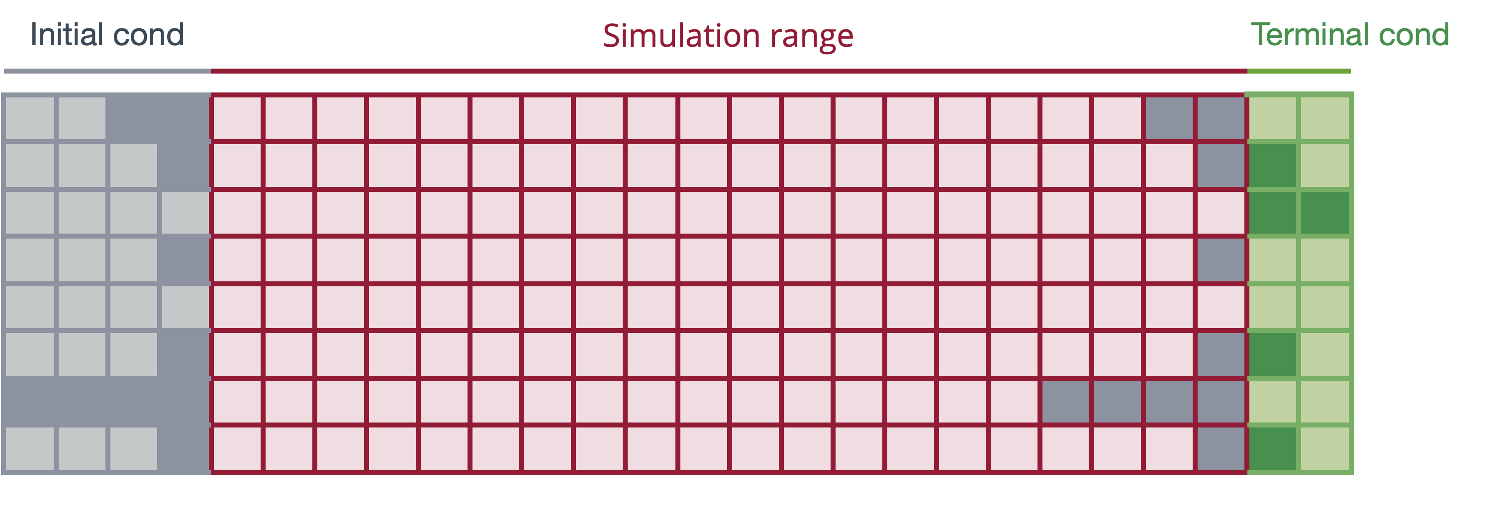
\[ \begin{gathered} f_1\left(x_{1-k}, \dots, x_{1+m} \right) = 0 \\[5pt] f_2\left(x_{1-k}, \dots, x_{1+m} \right) = 0 \\[5pt] \vdots \\[5pt] f_n\left(x_{1-k}, \dots, x_{1+m} \right) = 0 \\[5pt] \vdots \\[5pt] \vdots \\[5pt] f_1\left(x_{T-k}, \dots, x_{T+m} \right) = 0 \\[5pt] f_2\left(x_{T-k}, \dots, x_{T+m} \right) = 0 \\[5pt] \vdots \\[5pt] f_n\left(x_{T-k}, \dots, x_{T+m} \right) = 0 \end{gathered} \notag \]

Simulation setup

Initialize

Create an $n\times (T+k+m)$ matrix
Fill in initial condition in columns $1, \dots, k$

In each iteration

Fill in the simulation range columns
Taking the last simulation range columns as initial condition, use the first order simulator to fill in terminal codnition
Evaluate the LHS–RHS discrepancy for all $n\times T$ equations and send this information to the solver

Visualization of the simulation setup

Terminal condition derived from first-order solution

First-order solution of the model (model-consistent expectations of endogenous variables integrated away)

\[ x_t \approx T \ x_{t-1} + K + R_0 \ \varepsilon_t + \cdots + R_h \ \mathrm E_t \! \left[ \varepsilon_{t+h} \right] \notag \]

Create a stacked system to calculate the terminal condition points needed $$ \begin{bmatrix} x_{T+1} \[5pt] \vdots \[5pt] x_{T+m} \end{bmatrix} = T^\mathrm{term} \begin{bmatrix} x_{T+1-k} \[5pt] \vdots \[5pt] x_{T} \end{bmatrix} + K^\mathrm{term} \notag $$

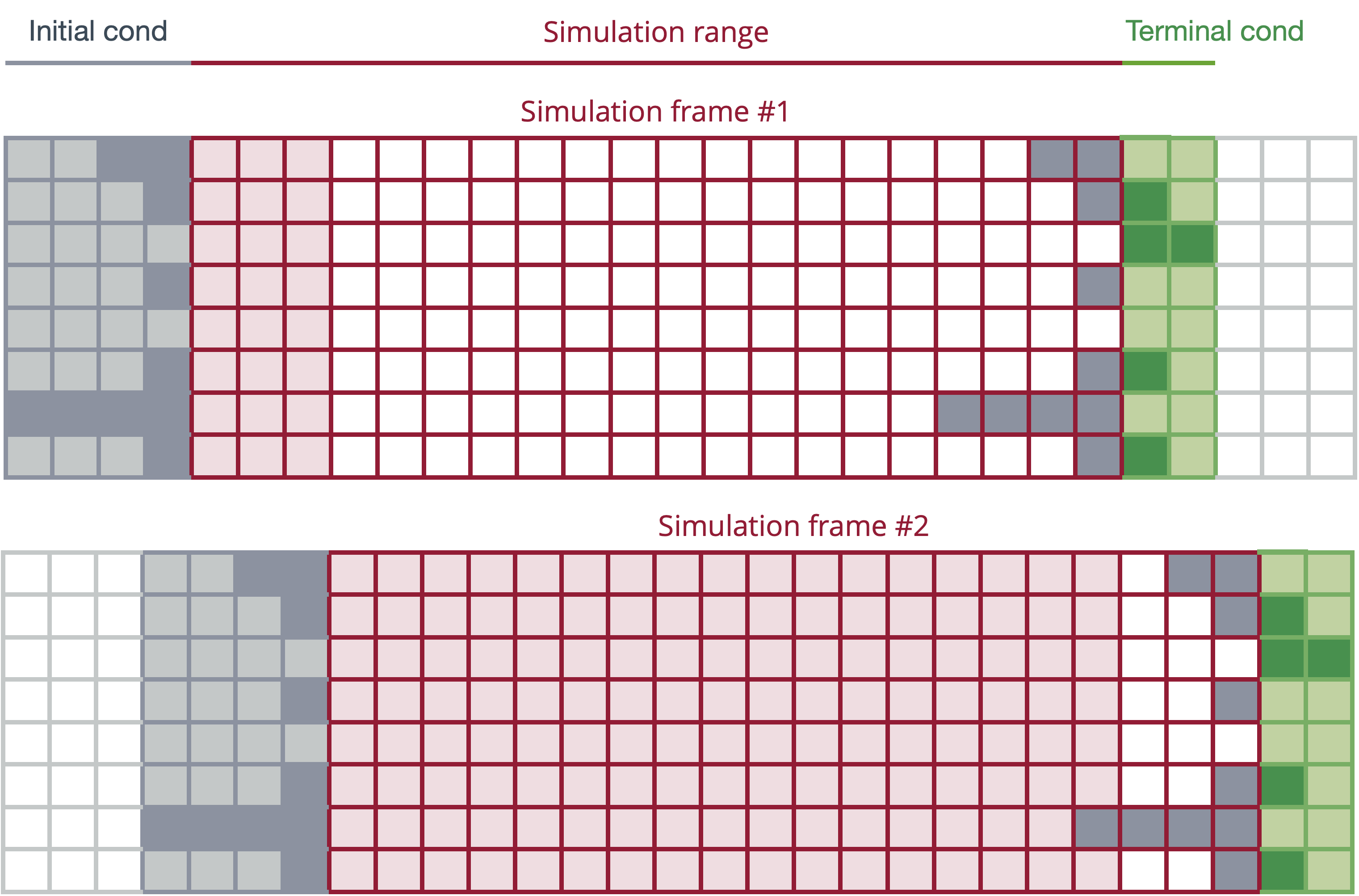
Changes in information sets within a simulation

By design, a stacked time simulation is consistent with an assumption of all future events (shocks, swaps) are anticipated
To simulate a sequence of unanticipated events, the simulation needs to be broken down into a sequence of sub-simulations (simulation frames)

Breakdown of simulation into frames

Implemenation in IrisT

Syntax of the simulate function for the stacked time method

[outputDb, info, frameDb] = simulate( ...
    model, inputDb, range ...
    , method="stacked" ...
);

Output structure info

Auxiliary output databank with simulation frames frameDb

Options to control the setup of the stacked time method

startIter=

"firstOrder" (default)
"data"

terminal=

"firstOrder" (default)
"data"